Plastics can be shaped into useful products using several different molding techniques, each suited for specific applications. Understanding these processes provides context for why injection molding is such a dominant method in industry today.

 

🔹 Overview of Common Molding Techniques

 

• Extrusion Molding: Plastic pellets are melted and forced continuously through a die to create long, uniform shapes such as pipes, sheets, and films. The process is best for continuous profiles rather than discrete parts.
• Injection Molding: Involves melting polymer pellets and injecting them under high pressure into a closed mold. After cooling and solidifying, the mold opens to eject the final part. This method is ideal for complex geometries and high-volume production.
• Compression Molding: Thermoset resins or elastomers are placed into a heated mold cavity and compressed until they take shape. It is widely used in automotive and aerospace industries for large, strong parts.
• Thermoforming: A sheet of thermoplastic is heated until soft and then shaped over a mold using vacuum or pressure. This technique is common for packaging materials, disposable cups, and trays.
• Rotational Molding: Powdered plastic is placed inside a hollow mold that rotates in an oven. The material melts and coats the mold’s interior, creating hollow products like tanks, toys, and containers.

 

While all of these techniques have their importance, injection molding remains the most versatile and widespread method due to its ability to produce detailed, high-precision parts in large volumes. The rest of this guide will focus on injection molding machines, their operation, and settings.

 

Main Parts of an Injection Molding Machine

 

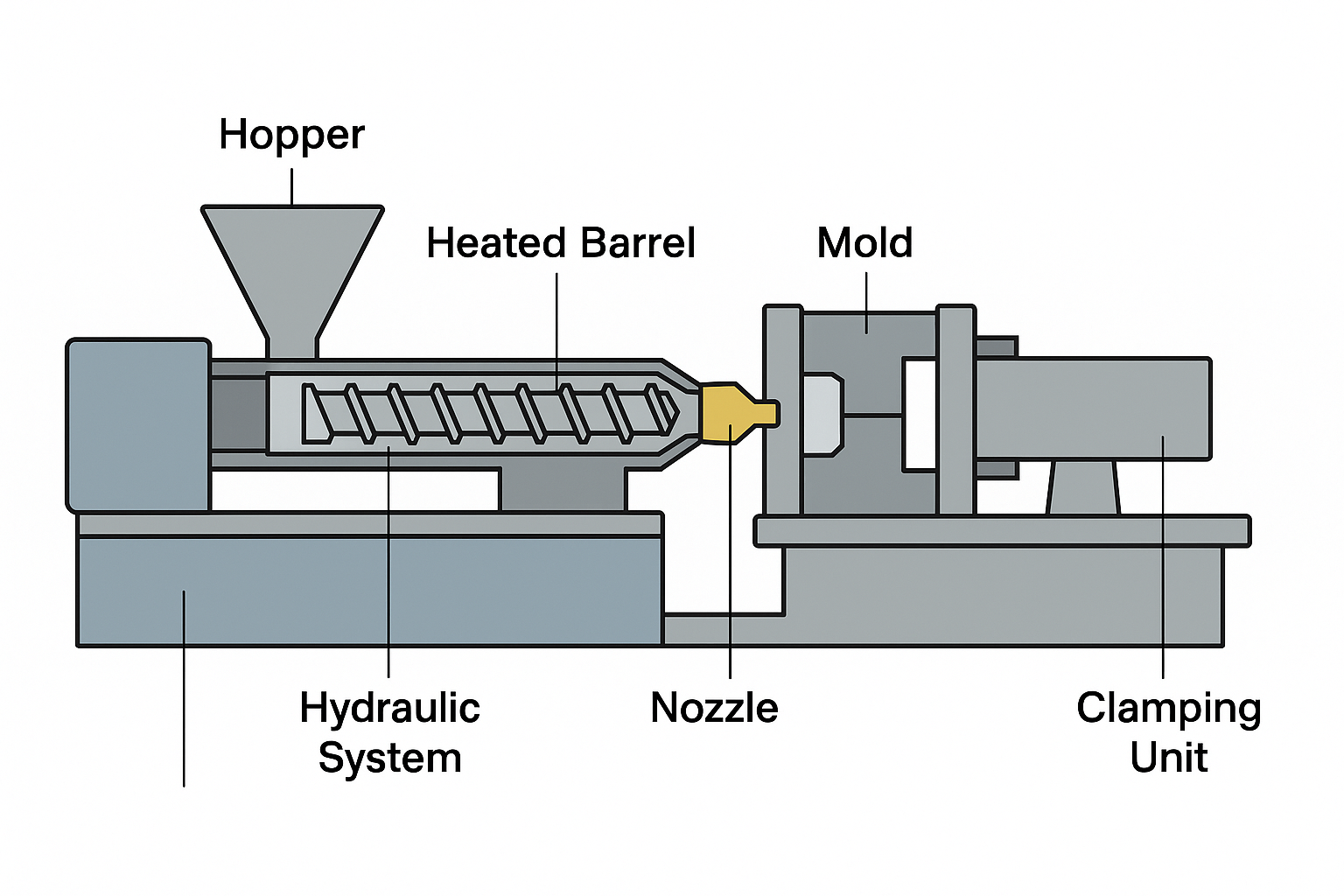
Below is a diagram labeling the essential components:

The machine consists of several critical sections. At the top is the hopper, which stores and delivers raw plastic pellets into the machine. The pellets then move into the heated barrel, where a rotating screw conveys them forward while gradually heating and melting the plastic. This combination of shear and heat ensures thorough melting and homogenization. The melted polymer is then pushed forward through the nozzle, which acts as the connection point between the injection unit and the mold. The mold is where the final part is shaped — molten plastic fills the cavity, cools, and solidifies to match the mold’s geometry. The clamping unit applies strong force to keep the mold halves shut during injection, preventing the material from leaking out. Finally, the hydraulic or electric drive system provides the power for screw rotation, injection, and clamping.

 

Understanding each part and its role is essential because any malfunction (like poor heating, low clamp force, or worn screws) will directly affect product quality.

 

Start-Up and Operation Procedure

 

Operating an injection molding machine involves a series of precise steps. Let’s expand on each:

 

1. Pre-Start Checks

Before switching on the machine, safety comes first. Operators should always wear heat-resistant gloves, safety glasses, and protective clothing. Next, all utilities such as hydraulic oil, cooling water, and compressed air must be verified. Without proper water flow, molds can overheat and damage. If using moisture-sensitive polymers like nylon or PET, proper drying in a hopper dryer is crucial to prevent degradation and poor part quality.

 

2. Machine Start-Up

Once utilities are confirmed, power on the machine and turn on heaters. It typically takes 20–30 minutes for the barrel zones and mold to stabilize at their set temperatures. During this period, the screw should be jogged gently after heating to ensure free rotation. Purging the barrel removes any residual material from previous runs, avoiding contamination and defects.

 

3. Mold Setup

The mold must be mounted securely and aligned in the clamping unit. Cooling lines are connected to regulate temperature, and electrical heaters or sensors are wired if needed. A mold safety check ensures the ejectors, guide pins, and parting line are working properly.

 

4. Setting Process Parameters

Operators set the barrel temperature profile, injection speed, pressure, holding time, and clamp force. Each setting must be chosen carefully to match the material’s processing window and the part’s requirements. Incorrect parameters can result in short shots, flashing, or part warpage.

 

Typical Settings for Different Polymers:

 

• Polypropylene (PP): Barrel 180–230 °C, Mold 30–60 °C, Injection Pressure 800–1200 bar, Injection Speed medium-high, Cooling 15–25 s.

 

• ABS: Barrel 200–250 °C, Mold 40–80 °C, Injection Pressure 1000–1500 bar, Injection Speed medium, Cooling 20–30 s.

 

• Polycarbonate (PC): Barrel 260–320 °C, Mold 80–120 °C, Injection Pressure 1200–1800 bar, Injection Speed medium-low, Cooling 25–40 s.

 

• Nylon (PA6): Barrel 230–280 °C, Mold 60–90 °C, Injection Pressure 1000–1500 bar, Injection Speed medium, Cooling 20–35 s.

 

• PET: Barrel 250–280 °C, Mold 90–120 °C, Injection Pressure 1200–1600 bar, Injection Speed high, Cooling 15–25 s (must be dried thoroughly).

 

5. Trial Shots

During initial runs, the mold is closed slowly in setup mode. Injection is done manually at lower speeds to prevent damage. Parts are inspected for quality defects such as weld lines, bubbles, or incomplete filling. Adjustments are made gradually.

 

6. Production Mode

Once stable, the machine is switched to automatic cycle mode. The process repeats: clamping, injecting, packing, cooling, opening, and ejection. Continuous monitoring is necessary to detect process drifts.

 

7. Shutdown

To shut down, stop feeding material, purge the barrel, and turn off heaters. Hydraulic pressure should be relieved, and the mold should be left open. The area must be cleaned, and records logged for future reference.

 

Temperature Profile Example

 

The temperature profile along the barrel is one of the most important settings. The rear zone must be lower to avoid premature softening or bridging of pellets, while the middle and front zones gradually increase to ensure full melting. The nozzle is often slightly cooler to prevent drooling of molten material.

 

Here’s a typical ABS temperature profile:

 

 

In this graph, we see the temperature gradually rising from the rear zone (200 °C) to the front zone (240 °C), then slightly decreasing at the nozzle (230 °C). This balance ensures smooth melting and avoids overheating or material degradation.

Injection Pressure Profile

 

Injection pressure is another critical variable. Too little pressure results in incomplete filling, while too much can cause flash, mold damage, or material stress. A controlled pressure profile helps balance flow and quality.

 

 

In this graph, the cycle is divided into four stages:

 

• Filling: Rapid rise in pressure pushes molten plastic into the mold cavity.
• Packing: High pressure is maintained to fill shrinkage and ensure complete part formation.
• Holding: Pressure gradually decreases to maintain the shape while preventing overpacking.
• Cooling: Pressure drops to zero as the part solidifies.

 

This staged approach prevents common defects like short shots, sink marks, or flashing.

Injection Speed

Injection speed controls how fast the molten plastic fills the mold cavity. High speeds are needed for thin-walled parts to avoid premature solidification, while lower speeds are preferred for thick parts to reduce stress and prevent flow marks.

 

• Thin parts → high speed (200–500 mm/s) ensures rapid filling.
• Thick parts → lower speed avoids voids and jetting.
• Amorphous plastics like ABS, PS, and PMMA generally tolerate higher speeds.
• Semi-crystalline plastics like PP, PA, and POM often require slower speeds to avoid defects.

 

Modern machines allow multi-stage speed control: starting fast to fill most of the cavity, then slowing down near the end to prevent defects at the gate or weld lines.

 

Typical Speed Guidelines for Common Polymers:

 

• PP: Medium-high speed, 80–150 mm/s.
• ABS: Medium speed, 60–120 mm/s.
• PC: Medium-low speed, 40–100 mm/s (to avoid stress).
• PA (Nylon): Medium speed, 70–120 mm/s.
• PET: High speed, 120–200 mm/s (thin-wall applications).

Machine Settings Checklist

 

The settings of an injection molding machine are interconnected. Here’s how each plays a role:

 

• Temperature: Determines melting and flowability of the resin.
• Injection Unit: Speed, injection pressure, holding pressure/time, screw speed, and back pressure all influence melt preparation and delivery.
• Clamping Unit: Clamp force prevents mold opening under cavity pressure, while ejector stroke and speed define how parts are removed.
• Cycle Timing: Each phase (injection, holding, cooling, mold open/close) is carefully timed to ensure repeatability.
• Safety Systems: Interlocks, decompression (suck-back), and alarms prevent accidents and material wastage.

 

Each parameter must be set based on material datasheets, mold design, and past process knowledge.

Mold Removal (Ejection) Types

 

Ejection of parts from the mold can be achieved in several ways:

 

• Ejector pins are the most common, pushing the part out with small round pins. They may leave minor marks.
• Sleeve ejection is used for cylindrical parts, like bottle caps, providing uniform removal force.
• Stripper plates push out thin or flat parts uniformly without pin marks.
• Air ejection blows compressed air between part and cavity to break suction.
• Unscrewing mechanisms are used for threaded parts, rotating the core to avoid damage.
• Robotic/manual removal handles delicate or complex shapes that require special care.

 

Each method is chosen depending on the geometry and precision requirements of the part.

⚠️ Disclaimer

All information provided in this blog is for educational purposes only. It is not intended for practical machine operation at home or without professional supervision. Injection molding machines operate at very high temperatures and pressures, making them dangerous if mishandled. We do not take responsibility for any consequences of using this data to run equipment.

Chemical bonds and the structure of molecules are ideas based on the modern atomic model. They help us understand how matter behaves and their chemical and physical properties.

 

What is a Chemical Bond?

 

Most atoms are not stable on their own, so they bind chemically with other atoms to become stable.

 

One of the most common ways atoms bond is through covalent bonding and understanding how it works gives us insight into the very structure of matter.

What is a Covalent Bond?

A covalent bond forms when two atoms share a pair of electrons. Each atom contributes one electron to the shared pair, creating a strong connection between them. This kind of bond can happen between atoms of the same element (like two oxygen atoms forming O₂) or between different elements (like hydrogen and oxygen forming H₂O).

 

But why do atoms share electrons in the first place?  Stability Through Sharing

Atoms are most stable when their outermost shell of electrons called the valence shell is full. Most elements aim to have eight electrons in their valence shell, a concept known as the octet rule.

 

For elements in the second period of the periodic table (like carbon, nitrogen, oxygen, and fluorine), achieving an octet (8 valence electrons) leads to high stability. These elements bond with others in ways that help them complete their octet.

While the octet rule works well for many elements, especially in the second period, there are exceptions.

1. Expanded Octets

Elements in the third period and beyond (like sulfur and phosphorus) have access to d orbitals in addition to s and p orbitals. This allows them to hold more than eight electrons in their valence shell.

 

Examples:

• SO₂ and SO₃ are molecules where sulfur has more than eight electrons around it.
• Sulfur can hold up to 18 electrons because of its 3d orbitals.

 

However, these d orbitals don’t always participate in bonding. In simple molecules like H₂S, sulfur still follows the octet rule without using its d orbitals.

2. Electron-Deficient Compounds

Some elements, especially beryllium (Be), boron (B), and aluminum (Al), often form compounds where the central atom ends up with fewer than eight electrons. These are known as electron-deficient molecules. These atoms still form stable compounds despite not completing an octet.

 

Examples:

• BeCl₂
• BH₃
• BCl₃
• AlCl₃

 

3. Odd-Electron Molecules

Not all molecules have an even number of electrons. Some, like nitric oxide (NO) and nitrogen dioxide (NO₂), have odd numbers of electrons. These compounds cannot complete the octet rule for all atoms involved but still exist and play important roles in chemistry and biology.

 

Special Case: Hydrogen

Hydrogen is a unique element. It has only one electron and just one orbital (1s), so it achieves stability with just two electrons. This is called the duet rule, and it’s why hydrogen only forms one covalent bond.

 

In Summary

• Covalent bonds involve sharing electrons to help atoms achieve stable electron configurations.
• Most atoms aim to follow the octet rule, but there are exceptions:
  • Expanded octets (elements with d orbitals)
  • Electron-deficient compounds (like those of B, Be, and Al)
  • Odd-electron molecules (like NO and NO₂)

 

What is a Lewis Dot Structures?

A Lewis dot diagram uses dots to represent valence electrons, the electrons in the outermost shell of an atom. These dots are placed around chemical symbols (like H, O, or Cl) to show how atoms share or transferelectrons when forming bonds.

 

A Lewis dot-dash structure is an extension of this idea, where a line (or dash) replaces a pair of bonding electrons between two atoms. This makes it easier to see single, double, or triple bonds.

 

How to Draw a Lewis Structure: The Step-by-steps

1. Identify the Central Atom

• Hydrogen and fluorine are usually not central atoms. They only form one bond.
• The less electronegative atom (less greedy for electrons) is typically at the center.

 Example: In H₂O, oxygen is in the center, and hydrogens are on the outside.

2. Count All Valence Electrons

Add up the valence electrons from each atom.

• For H₂O: O = 6 electrons, each H = 1 electron → 6 + 1 + 1 = 8 electrons
• For ions:
  • Add electrons for negative charges (like OH⁻: 6 + 1 + 1 = 8).
  • Subtract electrons for positive charges (like NH₄⁺: 5 + 4 – 1 = 8).

3. Create Single Bonds First

Connect each outer atom to the central atom with a pair of dots or a dash, representing one bond.

4. Complete the Octet Rule

Distribute the remaining electrons to satisfy the octet rule (8 electrons around each atom), starting with the most electronegative atom.

• For CCl₄, all four Cl atoms get three lone pairs (6 electrons each), and carbon forms four bonds (one with each Cl).

5. Check and Assign Formal Charges

Use this checklist:

• Lone pair? Both electrons go to that atom.
• Bonding pair? One electron goes to each atom.

Compare this to how many electrons the atom normally has. If it’s more or less, assign a formal charge.

Example: NH₂⁻ has a -1 charge on nitrogen because it appears to have one extra electron compared to its usual 5.

 

6. Rearranging for Stability

Sometimes the structure you first draw isn’t the most stable. You may need to:

• Convert lone pairs into bonding pairs to form double or triple bonds.
• Reduce formal charges across the molecule.

 

Example: For SO₃²⁻, you first draw 26 electrons. Then, adjust lone pairs to reduce charges and make a more stable structure. This might mean the sulfur ends up with more than 8 electrons—but that’s okay! Sulfur can expand its octet thanks to its d orbitals.

 

Special Notes:

• Hydrogen wants 2 electrons (not 8). It’s happy with just a duet.
• Elements beyond the second period (like sulfur and phosphorus) can hold more than 8 electrons.
• Electron-deficient elements (like Be, B, Al) can be stable with less than 8 electrons.
• Molecules like NO and NO₂ may have odd numbers of electrons and still exist stably.

 

Real-World Examples:

How Molecules Take Shape: Dative Bonds & VSEPR Theory Explained

 

What is a Dative Covalent Bond?  

Usually in covalent bonds, each atom shares one electron to form a shared pair. But sometimes, one atom donates both electrons and that’s when a dative covalent bond (also called a coordinate bond) is formed.

 How It Works:

• One atom has a lone pair (a non-bonded pair of electrons).
• Another atom has an empty orbital and needs electrons.
• The atom with the lone pair donates the entire pair into the empty orbital.
• This bond is often represented by an arrow (→) pointing from the donor to the acceptor.

 

Examples:

• NH₃ + BF₃ → H₃N→BF₃
  • Nitrogen has a lone pair.
  • Boron is electron deficient.
  • The arrow shows nitrogen donating a lone pair to boron.
• BH₃ reacting with CO or CN⁻ also creates similar dative bonds.

 

Dative Bonds in Complex Ions:

• Transition metals like Cu²⁺ can also form dative bonds.
• NH₃, H₂O, CO, or CN⁻ can donate lone pairs to the metal.
• This forms complex ions, where multiple dative bonds hold everything together.

 

 

VSEPR Theory: Predicting the Shape of Molecules

 (Valence Shell Electron Pair Repulsion Theory) Proposed by Gillespie and Nyholm, this theory says:

 

Electron pairs around a central atom will spread out as far as possible to minimize repulsion.

 

Types of Electron Pairs:

1. Bonding pairs – Electrons shared between two atoms.
2. Lone pairs – non-bonded electrons that stay with one atom.

 

Lone pairs repel more strongly than bonding pairs because they are only influenced by one nucleus.

 

Single, Double, and Triple Bonds:

• Each bond type (single, double, or triple) is treated as one repulsive unit (also called a VSEPR unit).
  • Example: CO₂ has two double bonds, so it has 2 VSEPR units.
  • Example: HCN has a triple bond between C and N, but still only 1 repulsive unit for that bond.

 

 Electron Pair Geometry vs. Molecular Shape:

There are three key terms you need to know:

Bond angles are included in the geometry, but not required when stating just the shape.

 

Repulsion Order:

When determining molecule shape, keep in mind:

 

This is why molecules like NH₃ and H₂O have less than ideal bond angles the lone pairs push the bonding pairs closer together.

 

VSEPR in Action:

Here’s a quick guide to the shapes based on the number of repulsive units:

From Atoms to Angles: How VSEPR Shapes Molecules

 

Let’s explore the main electron pair geometries and how they lead to different molecular shapes.

1. Linear Geometry

• Number of VSEPR units: 2
• Bond angle: 180°
• Example molecules: CO₂, BeCl₂

 Why it’s linear: The two bonding pairs of electrons stay as far apart as possible on opposite sides of the central atom forming a straight line.

2. Trigonal Planar Geometry

• Number of VSEPR units: 3
• Bond angle: 120°

All bonding pairs:

• Example: BF₃, SO₃, HCHO
• Shape: Trigonal planar

 

2 bonding + 1 lone pair:

• Example: SO₂
• Shape: Angular (Bent) due to lone pair repulsion

 Why it bends: The lone pair pushes the bonding pairs closer together, changing the shape.

3. Tetrahedral Geometry

 

• Number of VSEPR units: 4
• Bond angle: 109.5°

All bonding pairs:

• Example: CH₄
• Shape: Tetrahedral

 

3 bonding + 1 lone pair:

• Example: NH₃
• Shape: Trigonal pyramidal

2 bonding + 2 lone pairs:

• Example: H₂O
• Shape: Angular (Bent)

 

Note: As lone pairs increase, bond angles decrease due to increased repulsion.

4. Trigonal Bipyramidal Geometry

• Number of VSEPR units: 5

 

All bonding pairs:

• Example: PCl₅
• Shape: Trigonal bipyramidal

 

4 bonding + 1 lone pair:

• Example: SCl₄
• Shape: See-saw (Distorted tetrahedral)

 

3 bonding + 2 lone pairs:

• Example: ICl₃
• Shape: T-shaped

 

2 bonding + 3 lone pairs:

• Example: XeF₂
• Shape: Linear

Why shapes vary: Lone pairs take up more space, distorting ideal angles and leading to irregular shapes.

5. Octahedral Geometry

• Number of VSEPR units: 6
• Bond angle: 90°

 All bonding pairs:

• Example: SF₆
• Shape: Octahedral

5 bonding + 1 lone pair:

• Example: XeOF₄
• Shape: Distorted square pyramidal 

4 bonding + 2 lone pairs:

• Example: XeF₄
• Shape: Square planar

 

Visual trick: Connect all atoms with imaginary lines, and you’ll get 3D shapes like a pyramid, T-shape, or octahedron.

 

Quick Recap: VSEPR Shape Chart

 

Why Does This Matter?

The shape of a molecule affects:

• Polarity (whether a molecule has a positive and negative end)
• Reactivity (how it behaves in chemical reactions)
• Physical properties like boiling point, solubility, and more.

Introduction

Mechanical drawings are the language of engineering design. Whether you’re fabricating a machine part, constructing a plant layout, or designing a product assembly, mechanical drawings ensure everyone—from engineers to machinists—understands exactly what needs to be built.

In this post, we’ll explore the types of mechanical drawings, essential symbols and notations, and best practices for reading and creating technical drawings.

---

1.0 What Are Mechanical Drawings?

A mechanical drawing (also called an engineering drawing or technical drawing) is a precise, standardized representation of an object or system, created to communicate design intent. These drawings include:

• Dimensions

• Tolerances

• Material specifications

• Surface finishes

• Assembly instructions

They are used in mechanical, civil, structural, electrical, and manufacturing disciplines.

---

2.0 Types of Mechanical Drawings

Understanding the various types of mechanical drawings is essential for interpreting engineering documents:

1. Detail Drawings

• Focus on individual components

• Include dimensions, materials, surface finishes, and tolerances

• Used by machinists for part fabrication

2. Assembly Drawings

• Show how multiple parts fit together

• Include part numbers, exploded views, and fastening methods

• Often accompanied by a Bill of Materials (BOM)

3. Sectional Drawings

• Show interior details by cutting through an object

• Useful for complex parts that can’t be fully understood externally

4. Exploded Views

• Show components spaced out along an axis

• Ideal for understanding how parts assemble or disassemble

5. Isometric Drawings

• Represent 3D objects in 2D

• Common in plant layouts and piping diagrams

 

Example: Pressure Vessel Assembly Drawing Created Using SolidWorks

This detailed mechanical drawing illustrates the complete assembly of a pressure vessel, modeled and drafted in SolidWorks.

Figure: Isometric Assembly View of a Pressure Vessel

Figure: Vessel Drawing Front view, top view and side view

---

3.0 Common Symbols and Notations in Mechanical Drawings

Mechanical drawings use standardized symbols and conventions, as per ISO, ANSI, or ASME standards.

Note: Always refer to the title block for drawing-specific tolerances and scale.

---

4.0 Key Components of a Mechanical Drawing

1. Title Block

   • Contains drawing number, title, date, author, revision, material, and scale.

2. Views

   • Front, top, side, section, and isometric views for complete understanding.

3. Dimensions

   • Linear, radial, angular—always in standardized units (e.g., mm or inches).

4. Tolerances

   • Allowable variation in dimensions (important for manufacturability).

5. Bill of Materials (BOM)

   • List of parts used in an assembly drawing, with quantities and part numbers.

---

5.0 Best Practices for Reading Mechanical Drawings

• Start with the title block and scale.

• Identify main views (usually front view is most informative).

• Follow dimension lines and notes carefully.

• Review tolerances—they affect manufacturing and assembly.

• Study section views for hidden features.

• Look at material specifications and surface finish notes.

---

6.0 Best Practices for Creating Mechanical Drawings

1. Use Standard Templates – Stick to ISO or ASME drawing templates.

2. Ensure Clarity – Avoid crowding; use proper line types and scales.

3. Label Everything – Stream numbers, part names, notes, and units.

4. Maintain Consistency – Uniform font, arrowhead size, and dimensioning style.

5. Add Revision History – Track changes for version control.

6. Verify Against CAD Models – Always cross-check 2D with 3D models.

---

7.0 Software Tools for Mechanical Drawing

Modern mechanical drawings are created using CAD (Computer-Aided Design) software. Popular tools include:

• AutoCAD

• SolidWorks

• CATIA

• PTC Creo

• Fusion 360

• Inventor

These tools allow 2D drafting and 3D modeling, with built-in features for GD&T, BOMs, and simulations.

---

8.0 Why Mechanical Drawings Matter

Mechanical drawings ensure that what’s imagined can actually be manufactured. They:

• Reduce errors and miscommunication

• Standardize production and fabrication

• Serve as official documentation

• Enable collaboration across design, fabrication, and QA/QC teams

• Ensure compliance with codes and engineering standards

---

Conclusion

Whether you’re a design engineer, student, machinist, or project manager, understanding mechanical drawings is essential. They form the backbone of engineering design communication and ensure that products are built correctly and safely.

As you become more fluent in reading and creating these drawings, you’ll gain deeper insight into how machines and systems are conceived, designed, and brought to life.

The periodic table is more than a list of elements — it’s a powerful tool that reveals predictable patterns, or periodic trends, in the physical and chemical properties of elements. These trends arise from changes in atomic structure as we move across periods or down groups.

In this guide, we focus on the periodic trends shown by s- and p-block elements, following the Chemistry syllabus, including atomic and ionic sizes, ionization energy, electron gain energy, and electronegativity.

---

Sizes of Atoms and Ions

Atomic Size (Atomic Radius)

Atomic size refers to the distance between the nucleus and the outermost electron shell.

There are three commonly discussed atomic radii:

• Van der Waals Radius: Half the distance between two non-bonded atoms in neighboring molecules.

• Covalent Radius: Half the distance between two nuclei in a covalent bond.

• Metallic Radius: Half the distance between nuclei of two adjacent atoms in a metallic lattice.

📌 Covalent radius is typically used when discussing nonmetals; metallic radius for metals.

Periodic Trends in Atomic Radii

• Across a Period (→): Atomic radius decreases
  → Due to increasing nuclear charge pulling electrons closer.

• Down a Group (↓): Atomic radius increases
  → Due to addition of new electron shells.

---

Electron Configurations of Ions

When an atom loses electrons to form a cation, the electrons are removed first from the orbitals with the highest principal quantum number (n).
For instance, in a sodium atom with the configuration 1s² 2s² 2p⁶ 3s¹, the electron is lost from the 3s orbital, as it has the highest value of n.

When atoms become ions:

• Cations (positive ions): Lose electrons → become smaller
  → Sometimes lose an entire outer shell.

• Anions (negative ions): Gain electrons → become larger
  → Increased electron-electron repulsion expands the electron cloud.

Example:

• Na (Z = 11): 1s² 2s² 2p⁶ 3s¹
  → Na⁺ = 1s² 2s² 2p⁶ (smaller size)

• Cl (Z = 17): 1s² 2s² 2p⁶ 3s² 3p⁵
  → Cl⁻ = 1s² 2s² 2p⁶ 3s² 3p⁶ (larger size)

Periodic Trends in Ionic Radii

The radii of cations and anions, compared to their respective parent atoms (in picometres, pm), are shown in the figure below.

• Cationic radii are smaller than atomic radii.

• Anionic radii are larger than atomic radii.

• Across a period (for isoelectronic species): Ionic radii decrease with increasing nuclear charge.

• Down a group: Ionic radii increase due to added shells.

• An isoelectronic series refers to a group of atoms or ions that all have the same number of electrons.
  For example, the species O²⁻, F⁻, Ne, Na⁺, and Mg²⁺ each possess 10 electrons. Within such a series, as the atomic number increases, the nuclear charge also increases. Since the electron count stays the same, a stronger attraction is exerted by the nucleus on the electrons, causing the ionic radius to decrease progressively across the series.

---

Ionization Energy

Ionization energy (IE) is the energy required to remove one mole of electrons from one mole of gaseous atoms.

• The first ionization energy (I₁) is the energy needed to remove the outermost, most weakly held electron from a neutral atom in the gas phase. For instance, in the case of lithium, the first ionization involves the reaction:

Li(g) → Li⁺(g) + e⁻

• The second ionization energy (I₂) is the energy required to remove a second electron — this time from a positively charged ion (monovalent cation) to form a doubly charged ion (divalent cation). For lithium, this process is:

Li⁺(g) → Li²⁺(g) + e⁻

• Each successive ionization energy is higher than the previous one, as it’s increasingly difficult to remove electrons from an already positively charged ion.

• Ionization energy increases with each successive electron removed:
  I₁ < I₂ < I₃, and so on.

• Reason for the increase:
  Each electron is removed from a more positively charged ion, requiring more energy to overcome the stronger attraction to the nucleus.

• Sharp jump in ionization energy:
  A significant increase occurs when an inner-shell electron is removed after all outer-shell electrons have been taken.

• Why inner electrons require more energy:
  Inner-shell electrons are closer to the nucleus and experience a stronger electrostatic pull, making them harder to remove.

Periodic Trends in First Ionization Energies

• Across a Period: IE increases
  → Greater nuclear attraction and smaller size make it harder to remove electrons.

• Down a Group: IE decreases
  → Outer electrons are further from the nucleus and shielded by inner shells.

Detail diagrams of first ionization energy variation are given below.

Variation of First Ionization Energies Across Periods 1 and 2

The diagram shows how the first ionization energy changes as we move left to right across the first (H to He) and second (Li to Ne) periods of the periodic table.

Key Trends and Reasons:

• General Increase Across a Period:
  Ionization energy generally increases from left to right across both periods.
  🔹 This is because the nuclear charge increases (more protons in the nucleus), pulling electrons closer and more tightly, which makes them harder to remove.

• Same Shell, Increasing Attraction:
  Even though all elements in a period have electrons in the same principal energy level, the increasing nuclear charge leads to a stronger attraction, so more energy is required to remove an electron.

• Notable Exceptions:

  • Between Be and B, and N and O, there is a slight drop in ionization energy.

    • Boron vs. Beryllium: The 2p electron in boron is slightly easier to remove than the 2s electron in beryllium due to higher energy and shielding.

    • Oxygen vs. Nitrogen: In oxygen, electron pairing in the 2p orbital causes electron–electron repulsion, making it easier to remove one electron compared to nitrogen.

This pattern highlights how atomic structure, particularly nuclear charge and electron configuration, influences the energy needed to remove electrons, helping us understand chemical reactivity and periodic trends.

Note: Small dips occur due to electron pairing and subshell stability (e.g., Be vs. B, N vs. O).

---

Electron Gain Energy (Electron Affinity)

Electron gain energy refers to the energy change that occurs when an electron is added to a neutral atom in the gaseous state. For most elements, this process releases energy, meaning the value is negative.

For instance, when a chlorine atom gains an electron, it releases -349 kJ mol⁻¹, indicating that the process is energetically favorable:
Cl(g) + e⁻ → Cl⁻(g) ΔE EG = –349 kJ mol⁻¹

However, some atoms have positive electron gain energy values, such as beryllium (Be) and nitrogen (N).
This happens because:

• Be has a stable 2s² configuration.

• N has a half-filled 2p³ subshell.
  In both cases, adding another electron would cause electron–electron repulsion, making the process energetically unfavorable.

Examples:
N(g) + e⁻ → N⁻(g) ΔE EG = +134 kJ mol⁻¹
Be(g) + e⁻ → Be⁻(g) ΔE EG = +231 kJ mol⁻¹

Periodic Trends:

• Across a period: Electron gain energy becomes less positive (or more negative), meaning atoms are more likely to gain electrons.

• Down a group: It becomes more positive, indicating decreased tendency to accept electrons due to increased atomic size and shielding.

---

Relationship Between Electron Gain Energy and Electron Affinity

By international convention:

Electron gain energy (ΔE EG) = – Electron affinity (EA)

So, electron affinity represents the energy released when an electron is added to a gaseous atom, and it is numerically equal but opposite in sign to ΔE EG.

For example:
A⁻(g) → A(g) + e⁻ ΔE = EA,
which is the reverse of the electron gain process.

In summary, electron affinity is a key property that reflects how strongly an atom attracts an added electron and it closely mirrors the trends and behavior observed in electron gain energy.

• If energy is released, the value is negative → Atom strongly attracts electrons.

• If energy is absorbed, the value is positive → Atom resists gaining electrons.

Periodic Trends

• Across a Period: Electron gain energy becomes more negative (more exothermic).

• Down a Group: Becomes less negative → Larger atoms attract extra electrons less strongly.

📌 Halogens have the most negative electron affinities.
📌 Noble gases have positive electron gain energy — they don’t readily gain electrons.

---

Electronegativity

Electronegativity is the ability of an atom in a chemical bond to attract bonding electrons.

• Measured using Pauling scale (F = 3.98 is the highest).

• Not an actual energy value, but a relative scale.

The Role of Electronegativity in Chemical Bonding

Electronegativity is a key concept in chemistry—it helps us understand how atoms interact when they bond. By looking at the difference in electronegativity between two atoms, we can predict the type of bond they will form:

• Nonpolar covalent bond: Formed when the electronegativity difference is less than 0.4. Electrons are shared almost equally.

• Polar covalent bond: Occurs when the difference falls between 0.4 and 1.7. Electrons are shared unequally, creating partial charges on atoms.

• Ionic bond: Forms when the difference is greater than 1.7. One atom effectively takes an electron from the other.

Understanding this helps us predict a compound’s properties like polarity, solubility, and reactivity.

---

Electronegativity of Fluorine, Oxygen, and Chlorine

Among all elements, fluorine tops the electronegativity chart—it has the strongest tendency to attract electrons in a bond. Next comes oxygen, followed by chlorine.

What does this mean in practice?

• Fluorine is almost always assigned a negative oxidation state, no matter what it’s bonded to. Its extreme electronegativity makes it highly reactive—it aggressively pulls electrons toward itself.

• Oxygen also tends to be negative in compounds, except in rare cases like oxygen-fluorine compounds, where fluorine’s stronger pull takes precedence.

• Chlorine, while slightly less electronegative, still shows strong electron-attracting behavior, contributing to its reactivity in halogen reactions.

---

Why Noble Gases Don’t Have Electronegativity Values

You won’t find electronegativity values for noble gases (like helium, neon, or argon) on most charts. That’s because these elements don’t usually form chemical bonds—they already have full outer electron shells and are generally inert. Since electronegativity is about how strongly an atom attracts electrons in a bond, it doesn’t apply well to noble gases under normal conditions.

---

How to Determine the Electronegativity of a Molecule

To estimate the electronegativity behavior in a molecule, examine each individual bond:

1. Identify the two atoms involved in the bond.

2. Look up their electronegativity values (typically found on a periodic table).

3. Calculate the difference between the two.

The magnitude of this difference tells you how polar that bond is:

• Smaller difference → more equal sharing → nonpolar

• Larger difference → unequal sharing → polar or even ionic

This approach is especially useful in predicting molecular geometry, polarity, and how the molecule will interact with others (e.g., in solvents or reactions).

Periodic Trends

• Across a Period: Electronegativity increases
  → Due to smaller size and higher nuclear charge.

• Down a Group: Electronegativity decreases
  → Atoms are larger and exert weaker pull on bonding electrons.

---

Summary Table of Periodic Trends (s- and p-Block Elements)

---

Final Tips for Students

• Always relate trends to atomic structure: shell number, nuclear charge, and shielding.

• Practice comparing elements in same period or group.

• Be familiar with exceptions and reasons behind anomalies (like subshell stability).

• Link these trends to chemical properties such as reactivity, bonding, and compound formation.